1.6.1.1 The data🔗ℹ

R’s data(QuickStartExample) loads a list of x, 100 observations of 20 predictors, and y, a numeric response. glmnet/datasets loads it with one call, which returns both, as R’s x <- QuickStartExample$x; y <- QuickStartExample$y names them:

> (require glmnet/datasets glmnet/plot)

> (define-values (x y) (quick-start-example))

> x

#<design-matrix 100x20>

> (take (design-matrix-column-names x) 5)

'("V1" "V2" "V3" "V4" "V5")

> (take y 5)

'(-1.2748860319586857   1.8434251032391575   0.45923631556267985   0.5640407381654364   1.8729632580619755)

x is a design-matrix?. R’s matrix has no column names, and R’s coef calls its columns V1 to V20, as x names them.

1.6.1.2 The path🔗ℹ

R’s fit <- glmnet(x, y) fits the lasso over R’s automatic sequence of λ; elnet-path is its counterpart. R’s plot(fit) draws each coefficient against −log λ:

> (define fit (elnet-path x y))

> (plot-coefficient-path fit)

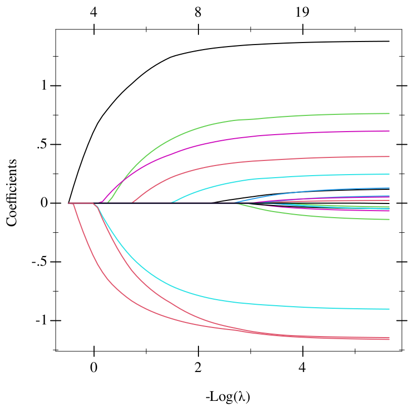
Each curve leaves zero where its predictor enters the model. The largest λ at which each coefficient is nonzero gives the order of entry:

> (define (entry-lambda j)     (for/first ([beta (in-vector (glmnet-path-coefficients fit))]                 [lam (in-vector (glmnet-path-lambda fit))]                 #:unless (zero? (vector-ref beta j)))       lam))

> (define entries     (sort (for/list ([name (in-list (design-matrix-column-names x))]                      [j (in-naturals)])             (cons name (entry-lambda j)))           > #:key cdr))

> (for/list ([entry (in-list entries)])     (cons (car entry) (/ (round (* 1000 (cdr entry))) 1000)))

'(("V1" . 1.486)   ("V14" . 1.486)   ("V5" . 0.933)   ("V20" . 0.933)   ("V6" . 0.85)   ("V3" . 0.706)   ("V8" . 0.443)   ("V11" . 0.211)   ("V7" . 0.1)   ("V10" . 0.069)   ("V15" . 0.063)   ("V13" . 0.052)   ("V2" . 0.048)   ("V12" . 0.048)   ("V18" . 0.048)   ("V4" . 0.043)   ("V16" . 0.033)   ("V17" . 0.027)   ("V9" . 0.023)   ("V19" . 0.006))

V1 and V14 enter first, at λ ≈ 1.49, then V5 and V20 at 0.93, V6 at 0.85 and V3 at 0.71; the other fourteen follow at smaller λ, in the same order as in R’s fit. The vignette’s text describes the older x axis, the L1 norm of the coefficients, which was R’s default before glmnet 4.1-9 and is #:xvar 'norm here (see The x axis).

Printing the path, R’s print(fit), gives R’s table: the number of nonzero coefficients, the percentage of deviance explained, and λ. The path has 67 rows; as in the vignette, only the first ten are shown:

> fit

#<glmnet-path:gaussian    Df  %Dev  Lambda 1   0  0.00 1.63100 2   2  5.53 1.48600 3   2 14.59 1.35400 4   2 22.11 1.23400 5   2 28.36 1.12400 6   2 33.54 1.02400 7   4 39.04 0.93320 8   5 45.60 0.85030 9   5 51.54 0.77470 10  6 57.35 0.70590 ...

The path stops at the 67th λ, 0.00351, with every predictor in the model and 91.32% of the deviance explained, because the deviance explained has stopped growing.

1.6.1.3 Coefficients and predictions🔗ℹ

R’s coef(fit, s = 0.1) gives the intercept and the 20 coefficients at λ = 0.1. That value is between two fitted ones, and the coefficients are interpolated between them, as R interpolates them:

> (coef fit #:lambda 0.1)

'#(0.15092807247412926    1.3205971945479142    0.0    0.6751102344847403    0.0    -0.8174115175489668    0.5214366714587341    0.004829335148616431    0.3194159167155697    0.0    0.0    0.14249851856673404    0.0    0.0    -1.0599787019192302    0.0    0.0    0.0    0.0    0.0    -1.0218737036830785)

R prints them as a sparse column, with the names and a dot for each zero. The nonzero ones, by name:

> (for/list ([name (in-list (cons "(Intercept)" (design-matrix-column-names x)))]              [b (in-vector (coef fit #:lambda 0.1))]              #:unless (zero? b))     (cons name b))

'(("(Intercept)" . 0.15092807247412926)   ("V1" . 1.3205971945479142)   ("V3" . 0.6751102344847403)   ("V5" . -0.8174115175489668)   ("V6" . 0.5214366714587341)   ("V7" . 0.004829335148616431)   ("V8" . 0.3194159167155697)   ("V11" . 0.14249851856673404)   ("V14" . -1.0599787019192302)   ("V20" . -1.0218737036830785))

Nine predictors are in the model at λ = 0.1. V7 has only just entered, at λ ≈ 0.1001, and its coefficient is 0.0048.

R’s predict(fit, newx = x[1:5,], s = c(0.1, 0.05)) predicts the first five observations at two values of λ. The vignette draws random new rows, which Racket cannot reproduce, so the new rows here are the first five of x; design-matrix-select-rows counts rows from 0:

> (define first-five (design-matrix-select-rows x '(0 1 2 3 4)))

> (predict fit first-five #:lambda '(0.1 0.05))

'((-1.3667606958778622    2.562379220607296    0.5650269394403127    1.922395960000674    1.4467743321267257)   (-1.336265196924594    2.589424524770471    0.5872868479973349    2.097722192283843    1.6436279924900774))

1.6.1.4 Cross-validation🔗ℹ

R’s cvfit <- cv.glmnet(x, y) assigns each observation to one of ten folds at random, with R’s random number generator. The vignette’s numbers therefore depend on R’s generator and its seed: with set.seed(123), R’s lambda.min is 0.06284, and another seed gives another value. Racket’s generator is not R’s, so it cannot draw R’s folds. The folds here are fixed instead: observation i is in fold i mod 10. R writes the same folds as foldid <- rep(1:10, length.out = 100), counted from 1, and with them cv.glmnet(x, y, foldid = foldid) gives the numbers below:

> (define fold-ids (for/list ([i (in-range (length y))]) (modulo i 10)))

> (take fold-ids 12)

'(0 1 2 3 4 5 6 7 8 9 0 1)

> (define cvfit (elnet-cv x y #:fold-ids fold-ids))

> cvfit

#<glmnet-cv:gaussian Mean-Squared Error         Lambda  Index  Measure       SE  Nonzero   min  0.06897     34    1.022  0.08208       10   1se   0.1323     27    1.095  0.09617        8>

The printed summary has the rows and columns of R’s print(cvfit), with two differences: the index of each λ counts from 0, and each number is rounded to four significant digits on its own, where R formats each column as a whole and can show a digit more. R’s plot(cvfit) draws the cross-validated mean squared error with one standard error above and below it, and a dotted line at each of lambda-min and lambda-1se:

> (plot-cv cvfit)

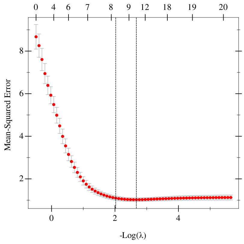
The error is smallest at λ = 0.06897, the 35th λ of the path, where ten predictors are in the model. lambda-1se, 0.1323, is the largest λ whose error is within one standard error of that minimum, 1.022 + 0.082: a simpler model, with eight predictors, whose error cannot be told apart from the best.

1.6.1.5 At lambda-min🔗ℹ

R’s cvfit$lambda.min, coef(cvfit, s = "lambda.min") and predict(cvfit, newx = x[1:5,], s = "lambda.min"). A cross-validated model’s coef and predict take 'lambda-min and 'lambda-1se for #:lambda, and default to 'lambda-1se, as R’s do:

> (glmnet-cv-lambda-min cvfit)

0.06896888915311372

> (coef cvfit #:lambda 'lambda-min)

'#(0.14792705583241395    1.3373939112007103    0.0    0.7040864806156394    0.0    -0.8428531496835723    0.5494034802965865    0.03270391434751026    0.34243052114343353    0.0    0.001206607686736499    0.1789959888283815    0.0    0.0    -1.0799934726815166    0.0    0.0    0.0    0.0    0.0    -1.0613824435251173)

> (predict cvfit first-five #:lambda 'lambda-min)

'(-1.3626976958215613   2.5736773620482443   0.5767334596516948   2.0062604430382738   1.541006086750126)

At lambda-min, V10 has joined the nine predictors of λ = 0.1, with a coefficient of 0.0012.

1.6.1.6 Matching R🔗ℹ

The same calls in R are

R 4.5.3 with glmnet 4.1.10 prints the same table, 67 rows from λ = 1.631 down to 0.003513, and gives the same coefficients and predictions, and lambda.min 0.06897 and lambda.1se 0.1323. The example’s companion test checks each number against R’s to six significant digits, and the parity tests ("vignette-*" in "scripts/r-parity/gen-reference.R") check the whole path, the printed table and the cross-validation to glmnet’s tolerances, on this dataset and on R glmnet’s six other example datasets.