1.6.4.1 The data🔗ℹ

The same fixture as Ridge regression (L2, α = 0): the response is exactly y = 1 + 2x₁ − x₂, and x₃ = x₁² is irrelevant.

> (define X '((1.0 2.0  1.0)               (2.0 1.0  4.0)               (3.0 4.0  9.0)               (4.0 3.0 16.0)               (5.0 6.0 25.0)               (6.0 5.0 36.0)))

> (define y '(1.0 4.0 3.0 6.0 5.0 8.0))

1.6.4.2 Fitting🔗ℹ

lasso is elnet-fit with #:alpha 1.0:

> (define fit (lasso X y #:lambda 0.05))

> (elnet-result-coefficients fit)

'#(1.8292174872340037 -0.8292174872340038 0.0)

The third coefficient is exactly 0.0: the irrelevant predictor has been selected out, while x₁ and x₂ keep their signs, a little shrunk. To list the predictors a fit kept:

> (for/list ([b (in-vector (elnet-result-coefficients fit))]              [j (in-naturals 1)]              #:unless (zero? b))     j)

'(1 2)

1.6.4.3 The selection path🔗ℹ

elnet-path fits a list of λ in one call, largest first (Regularization paths). Read upward, raising λ removes predictors one at a time:

> (define (round3 x)     (/ (round (* 1000 x)) 1000))

> (define (rounded v)     (for/list ([b (in-vector v)])       (round3 b)))

> (define path (elnet-path X y #:lambda '(0.01 0.05 0.2 0.5 1.0 2.5)))

> (for ([lam (in-vector (glmnet-path-lambda path))]         [beta (in-vector (glmnet-path-coefficients path))]         [r2 (in-vector (glmnet-path-dev-ratio path))])     (printf "λ = ~a: β = ~a, R² = ~a\n" lam (rounded beta) (round3 r2)))

λ = 2.5: β = (0.0 0.0 0.0), R² = 0.0 λ = 1.0: β = (0.586 0.0 0.0), R² = 0.611 λ = 0.5: β = (0.879 0.0 0.0), R² = 0.763 λ = 0.2: β = (1.317 -0.317 0.0), R² = 0.905 λ = 0.05: β = (1.829 -0.829 0.0), R² = 0.994 λ = 0.01: β = (1.96 -0.966 0.001), R² = 1.0

At λ = 0.01 all three predictors are in (the noise just barely); by λ = 0.05 x₃ is out; by λ = 0.5 x₂ is out; and at λ = 2.5 nothing is left. Once every coefficient is zero the fit is the intercept alone, which is the mean of the response:

> (elnet-result-intercept (lasso X y #:lambda 2.5))

4.499999999999999

plot-coefficient-path, from glmnet/plot, draws the same path as R’s plot(fit, label = TRUE) does (Coefficient paths): one curve per predictor against −log λ, so that the largest λ is at the left, with the count of nonzero coefficients along the top:

> (require glmnet/plot)

> (plot-coefficient-path path #:label #t)

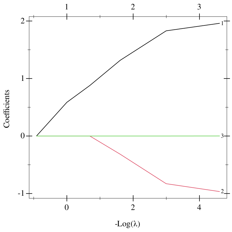
Read from the left, the plot is the table read from the top: x₁ enters at λ = 1, x₂ at λ = 0.2, and x₃ only at the smallest λ, 0.01, with a coefficient too small to lift its curve visibly off zero, although the count along the top reaches 3.

1.6.4.4 Choosing λ by cross-validation🔗ℹ

Six observations without noise are no test of λ: with no noise to overfit, the smallest λ predicts best. With noisy data, cross-validation chooses λ by how well each fit predicts observations it did not see (Choosing λ by cross-validation). Here are 40 observations of the same model, with uniform noise on [−1, 1] added to y:

> (random-seed 3)

> (define (uniform a b)     (+ a (* (- b a) (random))))

> (define X40     (for/list ([i (in-range 40)])       (define x1 (uniform 0 6))       (list x1 (uniform 0 6) (* x1 x1))))

> (define y40     (for/list ([row (in-list X40)])       (+ 1.0 (* 2 (car row)) (- (cadr row)) (uniform -1 1))))

> (define cv (elnet-cv X40 y40))

> cv

#<glmnet-cv:gaussian Mean-Squared Error         Lambda  Index  Measure       SE  Nonzero   min  0.01703     55   0.3378  0.05704        2   1se   0.1447     32    0.389  0.06871        2>

> (rounded (coef cv #:lambda 'lambda-min))

'(1.182 2.017 -1.061 0.0)

> (rounded (coef cv))

'(1.097 1.917 -0.949 0.0)

Both choices keep x₁ and x₂ and drop x₃. coef defaults to lambda-1se, the larger λ, whose coefficients are shrunk further from the true 2 and −1 in exchange for a model the data cannot tell apart from the best one.

plot-cv draws the cross-validated error as R’s plot(cvfit) does (Cross-validation curves):

> (plot-cv cv)

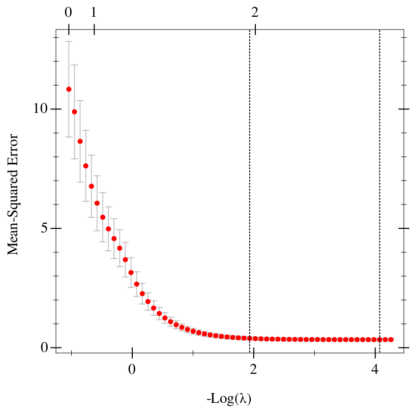
The red points are the error at each λ, with bars one standard error either side, and the dotted lines mark lambda-min, at the right, and lambda-1se, at the left. From lambda-1se rightwards every point lies within one standard error of the smallest error.

1.6.4.5 When to use it🔗ℹ

Use the lasso when you expect a sparse answer and want an interpretable list of predictors. Its weakness is correlated predictors: among a group that carries the same signal it tends to keep one arbitrarily and drop the rest. Elastic net (0 < α < 1) shows the problem and the fix.