1.6.11.1 The data🔗ℹ

glmnet/datasets provides R’s mtcars as a table: 32 cars from the 1974 Motor Trend road tests, with R’s eleven columns, among them miles per gallon ("mpg"), weight in thousands of pounds ("wt"), horsepower ("hp") and the quarter-mile time in seconds ("qsec"):

> (require glmnet/datasets)

> (table-column-names mtcars)

'("mpg" "cyl" "disp" "hp" "drat" "wt" "qsec" "vs" "am" "gear" "carb")

1.6.11.2 Crossing weight and horsepower🔗ℹ

(* wt hp) crosses the two columns: both main effects and their interaction, whose column is their product, named "wt:hp" as R names it:

> (define X (formula-design-matrix (~ mpg (* wt hp)) mtcars))

> (design-matrix-column-names X)

'("wt" "hp" "wt:hp")

> (design-matrix->rows (design-matrix-select-rows X '(0 1 2)))

'((2.62 110.0 288.2) (2.875 110.0 316.25) (2.32 93.0 215.76))

formula-path fits the lasso path on that design matrix:

> (define path (formula-path (~ mpg (* wt hp)) mtcars))

> (formula-model-predictor-names path)

'("wt" "hp" "wt:hp")

> (coef path #:lambda 0.5)

'(("(Intercept)" . 35.56562843492614)   ("wt" . -3.565144190560976)   ("hp" . -0.02730323502577826)   ("wt:hp" . 0.0))

> (coef path #:lambda 0.01)

'(("(Intercept)" . 48.48482015924476)   ("wt" . -7.765797007463395)   ("hp" . -0.11098237778796056)   ("wt:hp" . 0.02500290010294149))

Weight enters the path first. The interaction follows it, with a small negative coefficient, standing in for horsepower, which is still out; once horsepower enters, at λ ≈ 2.7, the interaction leaves again. At λ = 0.5 the lasso keeps weight and horsepower and leaves the interaction at zero. The interaction comes back below λ ≈ 0.10, now positive, and at λ = 0.01 its coefficient is about 0.025: each extra thousand pounds costs less fuel economy in a more powerful car. Weight and horsepower then have larger negative coefficients, which the positive interaction offsets. The plot of the path (Coefficient paths) shows where the interaction comes back:

> (require glmnet/plot)

> (plot-coefficient-path path #:label #t)

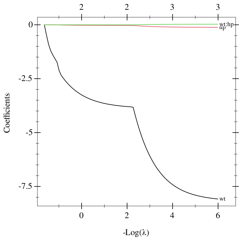
Near −log λ = 2.3, where the count along the top goes from 2 to 3, the weight’s curve turns sharply down, as the interaction takes over part of its effect. The interaction’s own curve stays close to zero on this scale, since its column, the product of weight and horsepower, is over a hundred times larger than the weight’s.

The infix spelling is the same formula, so it fits the same path:

> (mpg . ~ . wt * hp)

(~ mpg wt * hp)

> (equal? (formula-model-fit (formula-path (mpg . ~ . wt * hp) mtcars))           (formula-model-fit path))

#t

1.6.11.3 Every pair🔗ℹ

(^ (+ wt hp qsec) 2), R’s (wt + hp + qsec)^2, crosses the sum with itself: the three main effects, then the three two-way interactions, in R’s order.

> (define pairs-path (formula-path (~ mpg (^ (+ wt hp qsec) 2)) mtcars))

> (formula-model-predictor-names pairs-path)

'("wt" "hp" "qsec" "wt:hp" "wt:qsec" "hp:qsec")

> (coef pairs-path #:lambda 0.1)

'(("(Intercept)" . 24.780355625545575)   ("wt" . -3.1633077078543823)   ("hp" . 0.0)   ("qsec" . 0.7052063353878655)   ("wt:hp" . 0.002017087801293114)   ("wt:qsec" . -0.05663657693267714)   ("hp:qsec" . -0.001934541020569811))

At λ = 0.1 the lasso keeps weight, the quarter-mile time and all three interactions, and drops horsepower’s main effect: horsepower acts only through its interactions.

1.6.11.4 Choosing λ by cross-validation🔗ℹ

formula-cv cross-validates the crossed model. Four fixed folds, cars 0, 4, 8, … in the first, make the result the one R’s cv.glmnet(x, y, foldid = rep(1:4, length.out = 32)) gives:

> (define folds (for/list ([i (in-range 32)]) (modulo i 4)))

> (define cv (formula-cv (mpg . ~ . wt * hp) mtcars #:fold-ids folds))

> cv

#<glmnet-cv:gaussian (~ mpg wt * hp) Mean-Squared Error          Lambda  Index  Measure      SE  Nonzero   min  0.002503     82     6.08  0.6064        3   1se   0.04477     51     6.61  0.6951        3>

> (coef cv)

'(("(Intercept)" . 44.18599782499345)   ("wt" . -6.301381407673056)   ("hp" . -0.08130232129662496)   ("wt:hp" . 0.015743383605847892))

Both chosen λ values are below 0.10, where the interaction comes back, so both keep all three terms: every λ at which the interaction is out has a cross-validated error more than one standard error above the smallest. The model predicts from a new table, whose columns can come in any order; it computes the interaction itself:

> (define new-cars (list (cons "hp" '(100 200)) (cons "wt" '(2.5 3.5))))

> (predict cv new-cars)

'(24.238158077610287 16.89106716290629)

1.6.11.5 Matching R🔗ℹ

The same fits in R are

and R 4.5.3 with glmnet 4.1.10 gives the same path of 83 λ values, from 5.147 down to 0.002503, the coefficients above, and lambda.min 0.002503 and lambda.1se 0.04477. The example’s companion test checks each against R’s numbers to six significant digits.