1.5.2 Cross-validation curves🔗ℹ

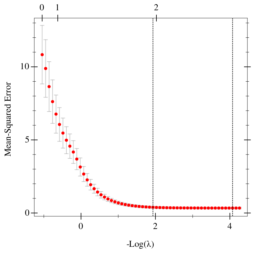
The lasso example cross-validates 40 observations of the fixture’s model, with noise added to y (see Choosing λ by cross-validation). plot-cv plots the result of elnet-cv as R’s plot(cvfit) does:

> (random-seed 3)

> (define (uniform a b)     (+ a (* (- b a) (random))))

> (define X40     (for/list ([i (in-range 40)])       (define x1 (uniform 0 6))       (list x1 (uniform 0 6) (* x1 x1))))

> (define y40     (for/list ([row (in-list X40)])       (+ 1.0 (* 2 (car row)) (- (cadr row)) (uniform -1 1))))

> (define cv (elnet-cv X40 y40))

> (plot-cv cv)

To read it:

• The red points are the cross-validated error, glmnet-cv-cvm, at each λ, and the grey bars reach from glmnet-cv-cvlo to glmnet-cv-cvup, one standard error either side. The y axis is labelled with R’s name for the measure, glmnet-cv-name.

• The x axis is −log λ, as in the path plot: heavy regularization at the left.

• The dotted lines mark the two choices. The right-hand one is lambda-min, where the error is smallest; the left-hand one is lambda-1se, the largest λ whose error is within one standard error of that smallest error.

• The axis along the top counts the nonzero coefficients, from glmnet-cv-nzero.

The error falls steeply while x₁ and x₂ enter, then flattens. From lambda-1se rightwards the curve stays within one standard error of its minimum, so the data cannot tell those models apart from the best one. lambda-1se is the simplest of them, which is why R’s predict and coef use it by default.

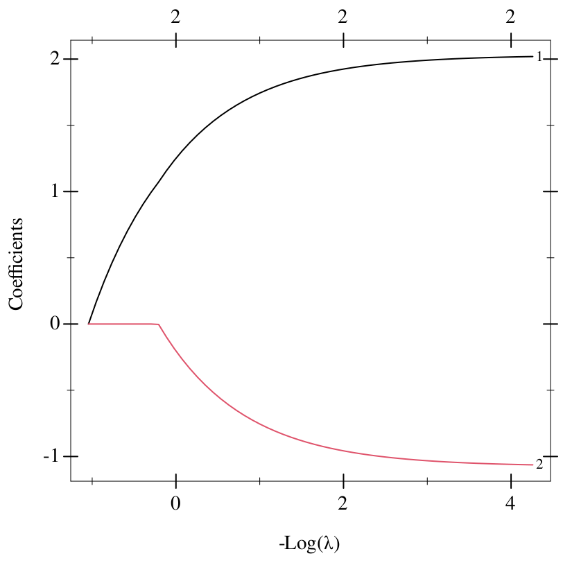
plot-coefficient-path plots the path of a glmnet-cv, the path fitted to all the data:

> (plot-coefficient-path cv #:label #t)