1.1.2 A First Regression
A fit is the result of solving an optimization problem on a dataset. For a Gaussian model, the objective described in the R glmnet vignette is:
minβ₀,β 1/(2n) ∑ᵢ₌₁ⁿ (yᵢ − β₀ − xᵢᵀβ)² + λ [α‖β‖₁ + (1−α)/2 ‖β‖₂²]
The solution gives the intercept β₀ and the predictor coefficients β. Here n is the number of observations, xᵢ holds the features for observation i, and yᵢ is its observed response. The parameter λ ≥ 0 controls the penalty’s strength, and α ∈ [0, 1] mixes the lasso and ridge penalties. Ordinary least squares (OLS) sets λ = 0, so only the squared-error term remains. See The penalty: α and λ for the other choices.
A design matrix X holds the predictors: one row per observation and one column per feature. The response y is separate, with one value per row. The library accepts lists or vectors of rows, or a design-matrix? value produced by one of its data adapters.
Start with R’s mtcars dataset: 32 cars with measurements of fuel economy and vehicle characteristics. We will predict fuel economy (mpg, miles per US gallon) from weight (wt, in thousands of pounds) and horsepower (hp). Load and display the Polars dataframe:
> (require datasets glmnet/data/polars (prefix-in pl: polars) racket/match) > (define cars (load-dataset 'mtcars #:format 'polars)) > cars
shape: (32, 12)
┌───────────────────┬──────┬─────┬───────┬───┬─────┬─────┬──────┬──────┐
│ model ┆ mpg ┆ cyl ┆ disp ┆ … ┆ vs ┆ am ┆ gear ┆ carb │
│ --- ┆ --- ┆ --- ┆ --- ┆ ┆ --- ┆ --- ┆ --- ┆ --- │
│ str ┆ f64 ┆ i64 ┆ f64 ┆ ┆ i64 ┆ i64 ┆ i64 ┆ i64 │
╞═══════════════════╪══════╪═════╪═══════╪═══╪═════╪═════╪══════╪══════╡
│ Mazda RX4 ┆ 21.0 ┆ 6 ┆ 160.0 ┆ … ┆ 0 ┆ 1 ┆ 4 ┆ 4 │
│ Mazda RX4 Wag ┆ 21.0 ┆ 6 ┆ 160.0 ┆ … ┆ 0 ┆ 1 ┆ 4 ┆ 4 │
│ Datsun 710 ┆ 22.8 ┆ 4 ┆ 108.0 ┆ … ┆ 1 ┆ 1 ┆ 4 ┆ 1 │
│ Hornet 4 Drive ┆ 21.4 ┆ 6 ┆ 258.0 ┆ … ┆ 1 ┆ 0 ┆ 3 ┆ 1 │
│ Hornet Sportabout ┆ 18.7 ┆ 8 ┆ 360.0 ┆ … ┆ 0 ┆ 0 ┆ 3 ┆ 2 │
│ … ┆ … ┆ … ┆ … ┆ … ┆ … ┆ … ┆ … ┆ … │
│ Lotus Europa ┆ 30.4 ┆ 4 ┆ 95.1 ┆ … ┆ 1 ┆ 1 ┆ 5 ┆ 2 │
│ Ford Pantera L ┆ 15.8 ┆ 8 ┆ 351.0 ┆ … ┆ 0 ┆ 1 ┆ 5 ┆ 4 │
│ Ferrari Dino ┆ 19.7 ┆ 6 ┆ 145.0 ┆ … ┆ 0 ┆ 1 ┆ 5 ┆ 6 │
│ Maserati Bora ┆ 15.0 ┆ 8 ┆ 301.0 ┆ … ┆ 0 ┆ 1 ┆ 5 ┆ 8 │
│ Volvo 142E ┆ 21.4 ┆ 4 ┆ 121.0 ┆ … ┆ 1 ┆ 1 ┆ 4 ┆ 2 │
└───────────────────┴──────┴─────┴───────┴───┴─────┴─────┴──────┴──────┘
The dataframe includes a text column, model, identifying each car. Select the two numeric predictors by name with polars->design-matrix, and extract the numeric response with polars->response:
> (define feature-names '("wt" "hp")) > (define X (polars->design-matrix cars feature-names)) > (define y (polars->response cars "mpg")) > (list (design-matrix-nrows X) (design-matrix-ncols X) (length y)) '(32 2 32)
ols fits a Gaussian model without a penalty. Fit it directly inside match-define. The and pattern binds the whole result as fit and extracts its intercept, coefficients, fraction of variance explained (R²), penalty strength, and number of solver passes:
> (match-define (and fit (elnet-result β₀ β R² λ n-steps)) (ols X y)) > fit #<glmnet:gaussian λ=0 dev=0.8268 nz=2/2>
> (list β₀ β R² λ n-steps)
'(37.22729275591213
#(-3.8778430581971657 -0.03177283120189043)
0.8267854518805285
0.0
15)
The intercept and coefficients describe the fitted linear relationship. With weight held constant, the horsepower coefficient describes the change in predicted fuel economy per additional horsepower; the weight coefficient holds horsepower constant. R² describes the fit to these observations, without estimating performance on new observations.
coef gives the intercept followed by the coefficients, in predictor column order, through the same interface for every family:
> (coef fit) '#(37.22729275591213 -3.8778430581971657 -0.03177283120189043)
To shrink the coefficients, fit the same data with a penalty. For example, lasso applies an L1 penalty and can set coefficients to zero:
> (define penalized-fit (lasso X y #:lambda 1.0)) > penalized-fit #<glmnet:gaussian λ=1 dev=0.7925 nz=2/2>
> (coef penalized-fit) '#(33.903898576422876 -3.2524096707366517 -0.02283397401445512)
Fit a regularization path to try many values of λ at once. elnet-path uses the lasso penalty by default. Its summary shows the number of nonzero coefficients, percentage of deviance explained, and λ for each fitted value:
> (define path (elnet-path X y #:nlambda 12)) > path
#<glmnet-path:gaussian
Df %Dev Lambda
1 0 0.00 5.1470
2 2 65.67 2.2280
3 2 79.49 0.9645
4 2 82.08 0.4175
5 2 82.57 0.1807
6 2 82.66 0.0782
7 2 82.67 0.0339
8 2 82.68 0.0147
9 2 82.68 0.0063>
To choose a penalty using held-out observations, elnet-cv cross-validates a path. It estimates prediction error at each λ and selects lambda.min and lambda.1se; Choosing λ by cross-validation explains how to use those results. For plots of paths and cross-validation curves, require glmnet/plot and see Plots.
1.1.2.1 Plotting the fit and path
Load glmnet/plot for coefficient paths and Racket’s plot for general plots. These examples return picts, which this manual and DrRacket display as images. plot-pict draws an image rather than opening a plot window.
> (require glmnet/plot plot)
1.1.2.1.1 Predicted versus actual values
Compare the OLS predictions with the observed responses. Points on the reference line have equal predicted and actual values:
> (define fitted (predict fit X))
> (plot-pict (list (function values #:color "gray" #:style 'short-dash) (points (map vector fitted y) #:alpha 0.5 #:size 3)) #:x-label "Predicted fuel economy (mpg)" #:y-label "Actual fuel economy (mpg)" #:title "Mtcars: OLS predicted vs actual" #:width 640 #:height 360)
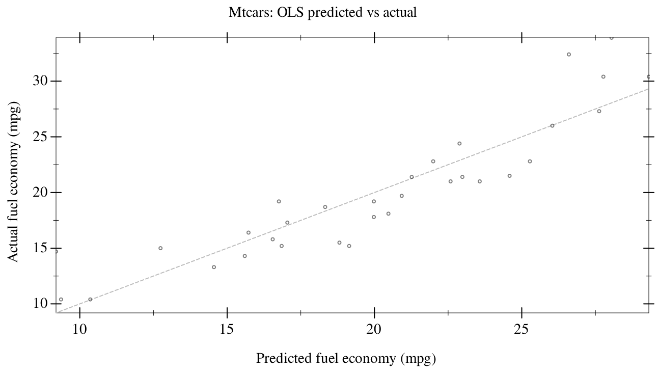
Points above the line are underpredictions; points below it are overpredictions. These predictions use the training observations, so this plot does not estimate prediction error on new data.
1.1.2.1.2 Residuals versus fitted values
For the OLS fit, a residual is the observed response minus its fitted value: rᵢ = yᵢ − ŷᵢ. Plot all 32 residuals against their fitted values, with a horizontal reference line at zero:
> (define residuals (map - y fitted))
> (plot-pict (list (hrule 0 #:color "gray" #:style 'short-dash) (points (map vector fitted residuals) #:alpha 0.5 #:size 3)) #:x-label "Fitted fuel economy (mpg)" #:y-label "Residual (observed - fitted)" #:title "Mtcars: OLS residuals vs fitted" #:width 640 #:height 360)
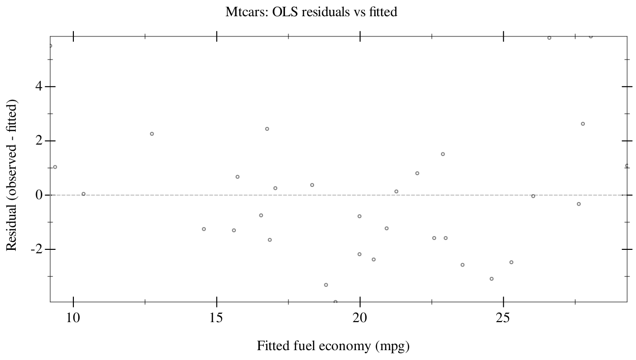
Curvature can suggest a missing nonlinear relationship; a widening spread can suggest that the residual variance changes with the fitted response. These are residuals on the training observations, so the plot is a model diagnostic rather than an estimate of prediction error on new data.
1.1.2.1.3 The lasso coefficient path
Fit a denser path to the same mtcars predictors and response, explicitly choosing the lasso penalty with #:alpha 1.0:
> (define lasso-path (elnet-path X y #:alpha 1.0))
> (plot-coefficient-path lasso-path #:label #t #:width 640 #:height 360 #:title "Mtcars: lasso coefficient path")
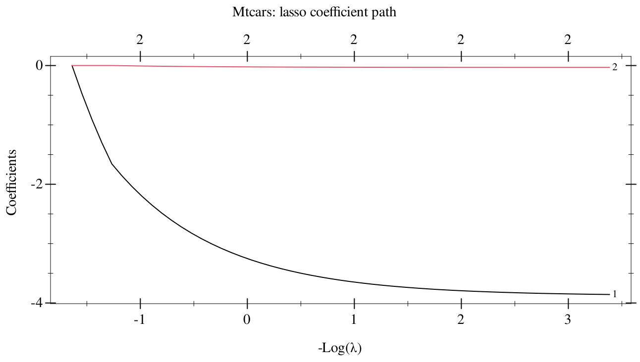
Each curve is a predictor’s coefficient as the penalty weakens from left to right. The horizontal axis is −log λ; the top axis counts the nonzero coefficients. The curve labels are predictor positions, starting at 1, in feature-names order. See Plots for other axis choices and cross-validation plots.