9.1 Distribution Objects🔗ℹ

A distribution object represents a probability distribution over a common domain, such as the real numbers, integers, or a set of symbols. Their constructors correspond with distribution families, such as the family of normal distributions.

A distribution object, or a value of type dist, has a density function (a pdf) and a procedure to generate random samples. An ordered distribution object, or a value of type ordered-dist, additionally has a cumulative distribution function (a cdf), and its generalized inverse (an inverse cdf).

The following example creates an ordered distribution object representing a normal distribution with mean 2 and standard deviation 5, computes an approximation of the probability of the half-open interval (1/2,1], and computes another approximation from random samples:
> (define d (normal-dist 2 5))
> (real-dist-prob d 0.5 1.0)

0.038651712749849576

> (define xs (sample d 10000))
> (fl (/ (count (λ (x) (and (1/2 . < . x) (x . <= . 1))) xs)
         (length xs)))

0.0391

This plots the pdf and a kernel density estimate of the pdf from random samples:
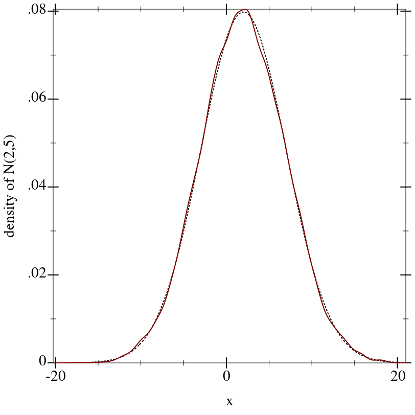
> (plot (list (function (distribution-pdf d) #:color 0 #:style 'dot)
              (density xs))
        #:x-label "x" #:y-label "density of N(2,5)")

image

There are also higher-order distributions, which take other distributions as constructor arguments. For example, the truncated distribution family returns a distribution like its distribution argument, but sets probability outside an interval to 0 and renormalizes the probabilities within the interval:
> (define d-trunc (truncated-dist d -inf.0 5))
> (real-dist-prob d-trunc 5 6)

0.0

> (real-dist-prob d-trunc 0.5 1.0)

0.0532578419490049

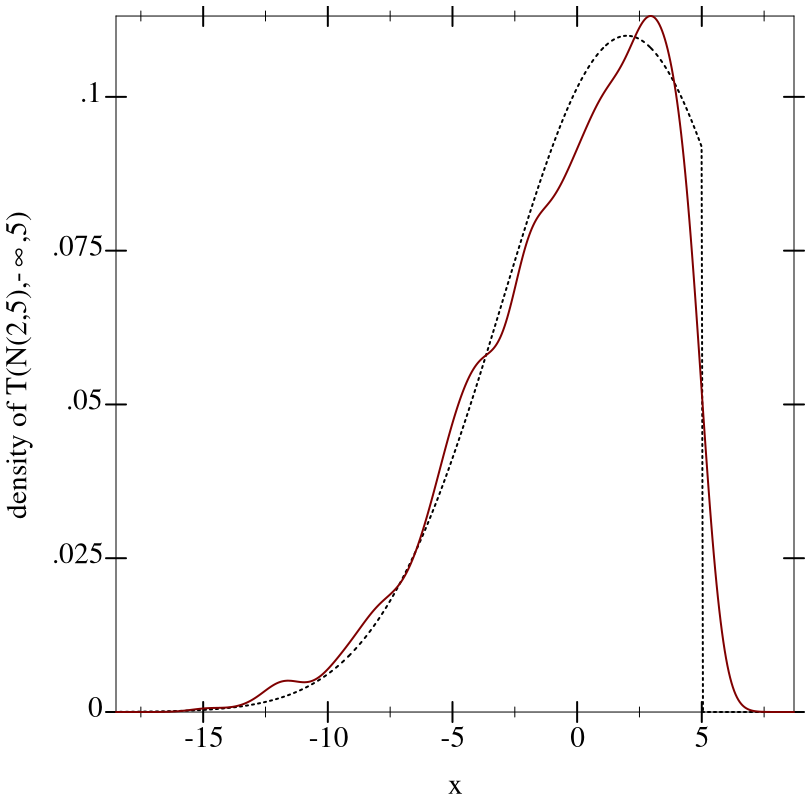
> (plot (list (function (distribution-pdf d-trunc) #:color 0 #:style 'dot)
              (density (sample d-trunc 1000)))
        #:x-label "x" #:y-label "density of T(N(2,5),-∞,5)")

image

Because real distributions’ cdfs represent the probability P[Xx], they are right-continuous (i.e. continuous from the right):
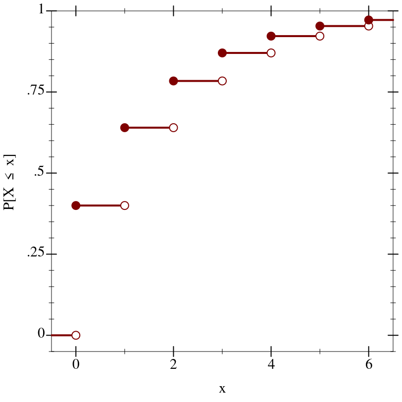
> (define d (geometric-dist 0.4))
> (plot (for/list ([i  (in-range -1 7)])
          (define i+1-ε (flprev (+ i 1.0)))
          (list (lines (list (vector i (cdf d i))
                             (vector i+1-ε (cdf d i+1-ε)))
                       #:width 2)
                (points (list (vector i (cdf d i)))
                        #:sym 'fullcircle5 #:color 1)
                (points (list (vector i+1-ε (cdf d i+1-ε)))
                        #:sym 'fullcircle5 #:color 1 #:fill-color 0)))
        #:x-min -0.5 #:x-max 6.5 #:y-min -0.05 #:y-max 1
        #:x-label "x" #:y-label "P[X ≤ x]")

image

For convenience, cdfs are defined over the extended reals regardless of their distribution’s support, but their inverses return values only within the support:
> (cdf d +inf.0)

1.0

> (cdf d 1.5)

0.64

> (cdf d -inf.0)

0.0

> (inv-cdf d (cdf d +inf.0))

+inf.0

> (inv-cdf d (cdf d 1.5))

1.0

> (inv-cdf d (cdf d -inf.0))

0.0

A distribution’s inverse cdf is defined on the interval [0,1] and is always left-continuous, except possibly at 0 when its support is bounded on the left (as with geometric-dist).

Every pdf and cdf can return log densities and log probabilities, in case densities or probabilities are too small to represent as flonums (i.e. are less than +min.0):
> (define d (normal-dist))
> (pdf d 40.0)

0.0

> (cdf d -40.0)

0.0

> (pdf d 40.0 #t)

-800.9189385332047

> (cdf d -40.0 #t)

-804.6084420137538

Additionally, every cdf can return upper-tail probabilities, which are always more accurate when lower-tail probabilities are greater than 0.5:
> (cdf d 20.0)

1.0

> (cdf d 20.0 #f #t)

2.7536241186062337e-89

Upper-tail probabilities can also be returned as log probabilities in case probabilities are too small:
> (cdf d 40.0)

1.0

> (cdf d 40.0 #f #t)

0.0

> (cdf d 40.0 #t #t)

-804.6084420137538

Inverse cdfs accept log probabilities and upper-tail probabilities.

The functions lg+ and lgsum, as well as others in math/flonum, perform arithmetic on log probabilities.

When distribution object constructors receive parameters outside their domains, they return undefined distributions, or distributions whose functions all return +nan.0:
> (pdf (gamma-dist -1 2) 2)

+nan.0

> (sample (poisson-dist -2))

+nan.0

> (cdf (beta-dist 0 0) 1/2)

+nan.0

> (inv-cdf (geometric-dist 1.1) 0.2)

+nan.0